OMX Drawing

Full Demo

This video provides a comprehensive overview of the system architecture and the end-to-end drawing process.

---

1. Overview

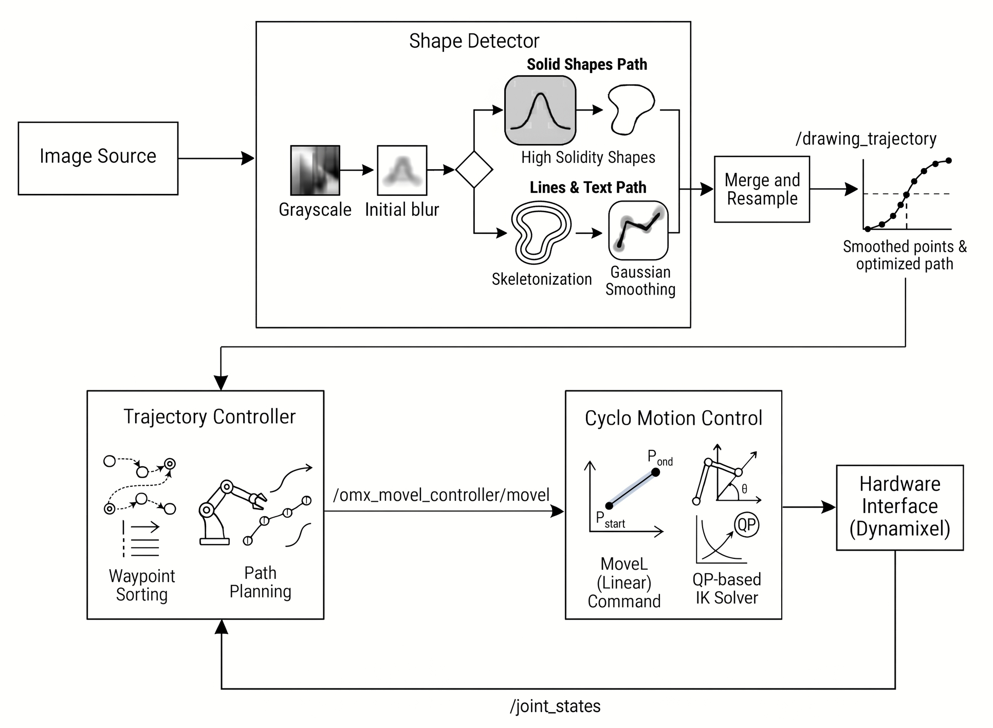
This project focuses on real-time end-effector trajectory control of the manipulator. The core components, shape_detector_node and omx_trajectory_controller_node, handle image processing and motion control respectively, operating harmoniously through ROS 2 topic communication.

Specifically, the shape_detector_node applies Adaptive Smoothing to extract high-precision trajectories from visual data. These extracted paths are then passed to the omx_trajectory_controller_node, which parses the robot's URDF during runtime to perform FK and IK internally, maintaining an independent control loop without relying on a separate high-level motion planning framework.

The pipeline utilizes Cyclo Control, a numerical Inverse Kinematics solver based on QP (Quadratic Programming) optimization, to calculate joint trajectories. Trajectory data from the vision node is processed through this controller and converted into real-time joint commands, ensuring smooth and precise motion on the drawing plane via a timer-based control loop.

Key Packages and File Structure

• scripts/shape_detector_node.py: Handles image preprocessing and trajectory extraction.
• scripts/omx_trajectory_controller_node.py: Handles trajectory reception and real-time motion control.
• launch/omx_drawing.launch.py: The launch file that integrates and runs the entire system.

---

2. Quick Start Guide

This guide provides a streamlined path to setting up and running the OMX drawing pipeline. Follow these phases to prepare your workspace, configure parameters, and execute the motion control using the official Cyclo Control framework.

Phase 1: Environment Setup & Build

Follow these steps in order to set up the official development environment and motion control packages.

# 1. Clone OpenManipulator Repository
cd ~
git clone https://github.com/ROBOTIS-GIT/open_manipulator.git

# 2. Enter Docker Container
cd ~/open_manipulator/docker
./container.sh start
./container.sh enter

# 3. Clone Cyclo Control in Workspace
cd ~/ros2_ws/src
git clone https://github.com/ROBOTIS-GIT/cyclo_control.git

# 4. Import Dependencies (Do not just clone)
vcs import . < cyclo_control/cyclo_control_ci.repos

# 5. Build the workspace
cd ~/ros2_ws
sudo apt update
rosdep install --from-paths src --ignore-src -r -y --rosdistro jazzy
colcon build --symlink-install --cmake-args -DCMAKE_BUILD_TYPE=Release
source install/setup.bash

Phase 2: Essential System Configuration (One-Time)

Apply optimized parameters directly using the following sed commands from your workspace root (~/ros2_ws).

1. TCP (Tool Center Point) Calibration Update the pen_link origin in the URDF to match the physical pen offset.

   sed -i '/<child link="end_effector_link"\/>/,/<\/joint>/ s/xyz=".*" rpy=".*"/xyz="0.01 0.015 0" rpy="0 0 -0.1571"/' \
   src/cyclo_control/cyclo_motion_controller_models/models/omx/omx_f.urdf

2. Dynamixel Hardware PID Tuning Align hardware response for high-friction drawing surfaces.

   sed -i 's/<parameter name="k_i">0<\/parameter>/<parameter name="k_i">1000<\/parameter>/g' \
   src/open_manipulator/open_manipulator_description/ros2_control/omx_f.ros2_control.xacro
   sed -i 's/<parameter name="k_d">1000<\/parameter>/<parameter name="k_d">1200<\/parameter>/g' \
   src/open_manipulator/open_manipulator_description/ros2_control/omx_f.ros2_control.xacro

3. Cyclo Control Gain Optimization Prioritize position tracking accuracy in task space.

   sed -i 's/weight_task_position: .*/weight_task_position: 1500.0/' \
   src/cyclo_control/cyclo_motion_controller_ros/config/omx_config.yaml

4. Collision Constraint Optimization for QP Solver

   sed -i 's/<collision>/<!-- <collision>/g; s/<\/collision>/<\/collision> -->/g' \
   src/cyclo_control/cyclo_motion_controller_models/models/omx/omx_f.urdf

   Note on Safety: Since software-level collision avoidance is disabled for this performance optimization, please ensure the robot's workspace is clear of obstacles and closely monitor the robot during operation to prevent physical collisions.

Phase 3: Execution & Verification

Run the drawing pipeline in three simple stages. Each terminal must enter the Docker container (./container.sh enter) first. Ensure you have sourced your workspace in each terminal.

1. Bring up OMX Hardware (Terminal 1)

   # Use the AI-optimized follower bringup
   ros2 launch open_manipulator_bringup omx_f.launch.py start_rviz:=true use_mock_hardware:=true

   Note: This setup is configured for simulation in RViz using mock hardware. To run it on actual hardware, execute the command without the start_rviz:=true and use_mock_hardware:=true flags.

2. Start Cyclo Control (Terminal 2) Launch the controller with interactive markers enabled for manual testing.

   ros2 launch cyclo_motion_controller_ros omx_controller.launch.py start_interactive_marker:=true

3. Launch Drawing Pipeline (Terminal 3)

   ros2 launch open_manipulator_playground omx_drawing.launch.py

---

3. Kinematic Background

The core of manipulator control is defining the relationship between each joint angle of the robot and the physical position of the end-effector.

3.1 Forward Kinematics (FK) vs Inverse Kinematics (IK)

Category	Forward Kinematics (FK)	Inverse Kinematics (IK)
Input	Joint angles (q)	Target end-effector pose (x_d)
Output	End-effector position and orientation (x)	Joint angles (q)
Mapping Direction	Joint Space → Task Space	Task Space → Joint Space
Uniqueness of Solution	Unique solution always exists	Multiple solutions may exist, or none
Computational Complexity	Relatively simple matrix operations	Numerical methods or optimization needed
Role in Control	State evaluation and visualization	Real-time control and trajectory tracking

3.2 Accurate Pen Tip Position Tracking via Pen_Link Addition

The Jacobian matrix provides a differential mapping that converts minute changes in Joint Space into Task Space velocities, which forms the core of task space control. In this drawing system, the geometric Jacobian is recalculated at every control step by parsing the modified URDF model at runtime, and this is shared across both forward and inverse kinematics operations.

▼ Click to view Advanced TCP Definition and URDF details

Advanced TCP (Tool Center Point) Definition via Virtual Link

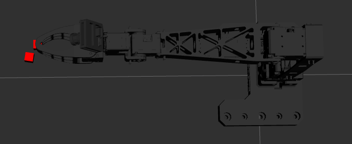
Standard robot models generally define the center of the gripper as the end-effector. However, for precise drawing using a pen, the position of the pen tip extending from the hardware mount must be the reference point for control (TCP). To achieve this, a hierarchical link structure starting from end_effector_link needs to be added to the URDF, considering the actual location where the pen tip is attached.

Physical Pen Setup	RViz Pen Link Visualization

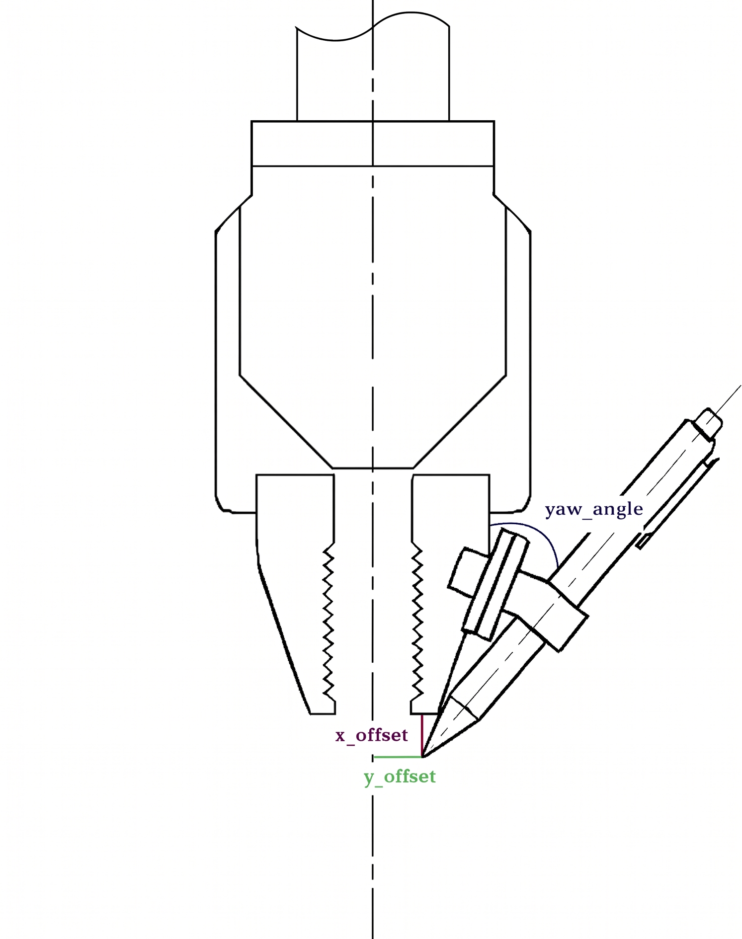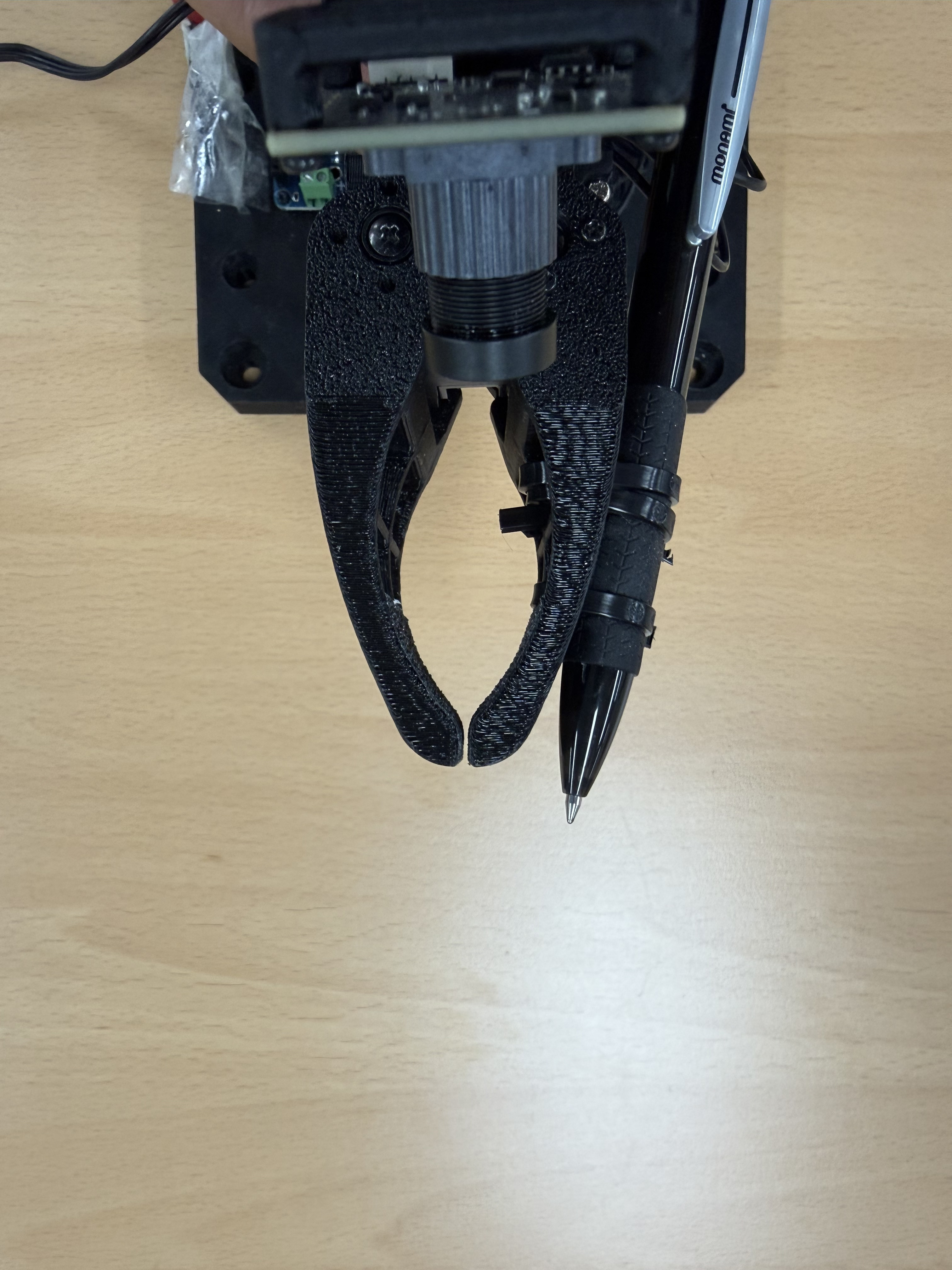<!-- 1. Existing end-effector (gripper center) definition -->
<joint name="end_effector_joint" type="fixed">
  <parent link="link5"/>
  <child link="end_effector_link"/>
  <origin rpy="0 0 0" xyz="0.09193 -0.0016 0"/>
</joint>
<link name="end_effector_link">
  <visual>
    <origin rpy="0 0 0" xyz="0 0 0"/>
    <geometry><box size="0.01 0.01 0.01"/></geometry>
    <material name="red"><color rgba="1.0 0.0 0.0 1"/></material>
  </visual>
</link>

<!-- 2. Added Pen Tip TCP definition -->
<joint name="pen_joint" type="fixed">
  <parent link="end_effector_link"/>
  <child link="pen_link"/>
  <origin rpy="0 0 -0.1571" xyz="0.01 0.015 0"/>
</joint>
<link name="pen_link">
  <visual>
    <origin rpy="0 0 0" xyz="0 0 0"/>
    <geometry><box size="0.01 0.01 0.01"/></geometry>
    <material name="red"><color rgba="1.0 0.0 0.0 1"/></material>
  </visual>
</link>

Original URDF File Path

ros2_ws/src/cyclo_control/cyclo_motion_controller_models/models/omx/omx_f.urdf

With this modification, the IK solver now computes joint angles targeting the coordinates of pen_link, which actually touches the paper, rather than the center of end_effector_link. The core of the high-precision drawing implemented in this project lies in the following measurement-based calibration.

1. Applying Measured Parameters: The origin data (xyz="0.01 0.015 0" rpy="0 0 -0.1571") of the pen_joint is not a simple estimate. It is the result of precisely and physically measuring the x_offset (10mm), y_offset (15mm), and the pen's tilt Yaw_angle (-9 degrees) of the pen attached to the actual hardware.

2. Hierarchical Calibration: The end_effector_link -> pen_link tree structure allows intuitive projection of physical measurements into the model, and even if the mounting state changes, immediate response is possible simply by modifying the URDF parameters.

3. Maximizing IK Precision: By synchronizing the error between the hardware and the virtual model to sub-millimeter levels, the 2D plane tracking performance of the pen tip can be maximized without additional compensation calculations at the algorithm stage.

4. Visual Debugging: By adding visualization elements (<visual>) to the virtual link, you can verify in real-time whether the pen tip's position in RViz matches the actual hardware. Use the command below to instantly verify if the modified URDF reflects your intentions visually.

   ros2 launch cyclo_motion_controller_models view_omx_f.launch.py

Stable Real-Time Control Based on QP Optimization

To ensure stability in a real-time execution environment, the inverse kinematics problem is solved using a QP (Quadratic Programming) optimization approach. By directly reflecting joint limits as constraints, it ensures the physical safety of the hardware while enabling smooth and reliable drawing trajectory tracking.

Relaxing Collision Constraints for QP Solver Optimization

The QP (Quadratic Programming) optimization-based solver calculates joint limits and distance constraints in real-time to find the optimal path. If complex collision tags are active in the URDF model, they can unnecessarily increase computational load or cause unintended self-collision constraints that may block motion during precise drawing. Therefore, to ensure smooth drawing execution, it is recommended to disable collision conditions for links by commenting out their collision tags, as shown in the example below.

<link name="link1">
  <visual>
    <origin rpy="0 0 0" xyz="0 0 0"/>
    <geometry>
      <mesh filename="package://open_manipulator_description/meshes/omx_f/follower_01_base.stl" scale="0.001 0.001 0.001"/>
    </geometry>
  </visual>
  <!-- Comment out collision tags using complex mesh data to reduce QP solver load. -->
  <!-- <collision>
    <origin rpy="0 0 0" xyz="0 0 0"/>
    <geometry>
      <mesh filename="package://open_manipulator_description/meshes/omx_f/follower_01_base.stl" scale="0.001 0.001 0.001"/>
    </geometry>
  </collision> -->
</link>

---

4. Controller and Motion Control Parameter Optimization

For precise drawing, consistent parameter optimization from the hardware interface to the high-level controller is essential. This section details the key settings modified for high-performance trajectory tracking and the reasoning behind their optimization.

4.1 Cyclo Control and Real-Time Controller Settings

The omx_movel_controller is responsible for the linear movement of the end-effector. To maximize drawing precision and hardware safety, its parameters have been optimized as follows:

▼ Click to view Detailed Parameter Explanation

omx_movel_controller:
  ros__parameters:
    control_frequency: 100.0        # Control loop frequency (Hz)
    time_step: 0.01                 # Computation timestep (1/frequency)
    
    kp_position: 50.0               # Task space position gain
    kp_orientation: 50.0            # Task space orientation gain

    weight_task_position: 1500.0    # Position tracking weight (Core for high-precision drawing)
    weight_task_orientation: 1.0    # Orientation maintenance weight
    weight_damping: 0.001           # Damping weight to avoid singularities
    slack_penalty: 1000.0           # Constraint relaxation penalty (Optimization stability)
    
    cbf_alpha: 5.0                  # CBF (Control Barrier Function) strength
    collision_buffer: 0.01          # Collision prevention buffer (m)
    collision_safe_distance: 0.005  # Collision safe distance (m)

    controlled_link: "pen_link"     # Target link to control (TCP)

Original Configuration File Path

ros2_ws/src/cyclo_control/cyclo_motion_controller_ros/config/omx_config.yaml

Detailed Parameter Explanation

1. Control Performance and Tracking

   • Weight Task Position (1500.0): Sets the position tracking weight in the task space very high, making it the top priority for the robot to accurately follow the input drawing trajectory over other secondary constraints.
   • KP Position/Orientation (50.0): The key gain for converting position/orientation errors in task space into linear and angular velocity commands, respectively. Similar to generating velocity commands to reach a target point in mobile base control, it acts as an intermediary to generate a virtual velocity vector so the end-effector can track the trajectory.
   • Controlled Link (pen_link): Sets the previously defined virtual pen tip link as the control reference, performing precise drawing by minimizing physical errors.

2. Optimization and Stability

   • Weight Damping (0.001): A damping component to increase the stability of the control loop and suppress minute motor vibrations (jitter).

3. Interface Topic Configuration

   • Joint States Topic (/joint_states): Receives the current joint state of the robot.
   • Joint Command Topic (/leader/joint_trajectory): Sends calculated joint trajectory commands to the lower-level controller (ros2_control).
   • MoveL Topic (~/movel): A topic that receives linear movement commands.
   • EE Pose Topic (~/current_pose): Publishes the current pose of the end-effector in real-time to assist with monitoring.
   • Controller Error Topic (~/controller_error): A topic for monitoring the tracking error with the target trajectory in real-time.

4.2 ros2_control and Dynamixel PID Tuning

PID and profile parameters have also been optimized at the Dynamixel hardware level for rapid and precise response.

Original URDF File Path

open_manipulator_description/ros2_control/omx_f.ros2_control.xacro

Item	Before (Default)	After (Optimized)	Role and Reason for Optimization
Position I Gain	0	1000	Eliminates steady-state error and overcomes frictional resistance
Position D Gain	1000	1200	Suppresses overshoot and vibration by improving braking performance

• I Gain: Ensures that the target coordinates are perfectly reached despite the slight friction generated when the pen tip touches the paper.
• D Gain: Minimizes shaking during high-speed movements and sudden changes in direction.

---

5. Software Detailed Configuration and Algorithms

These are the detailed technical specifications of the vision processing and motion control algorithms.

5.1 Vision Recognition and Data Preprocessing (Shape Detector Node)

shape_detector_node.py extracts precise linear data from the input image, considering the mechanical characteristics of the robot and the quality of the drawing.

▼ Click to view detailed Step-by-Step Vision Pipeline

Image Designed by Freepik

1. Step 1 (Image Analysis and Preprocessing):

   • Bilateral Filter: Unlike simple Gaussian blur, it effectively removes only noise while preserving edge information.
   • Adaptive Thresholding: Performs robust binarization against lighting changes, and uses Morphological Closing operations to fill broken lines or tiny gaps in text, ensuring structural integrity.

   

2. Step 2 (Skeletonization and Single Line Extraction):

   • Skeletonization: Converts the binarized outline into a 1-pixel thick centerline, extracting only the geometric skeleton.

• Line Extraction (Pixel Sorting): To extract valid point cloud data that the robot can follow without interruption, it applies a sorting algorithm (extract_single_line) based on Nearest Neighbor to the skeletonized pixels. By calculating the Euclidean distance between pixels, it sequentially connects the closest unvisited pixel within a threshold (50px²) from the current position.
• Segment Generation: The connected pixels are grouped into a single valid stroke sector that the robot can follow without stopping. If there are no neighboring pixels within the threshold, a new segment is created to prevent sudden jumps or discontinuities.

3. Step 3 (Adaptive Smoothing & Optimization):
   • Douglas-Peucker Algorithm: Detects vertices with sharp curvature across the entire trajectory. This preserves straight sections and selectively applies smoothing only to curved sections, preventing them from becoming blunt.
   • Trajectory Stitching: If the distance between two adjacent trajectories is within 25mm, they are forcibly merged into one continuous path, minimizing unnecessary pen-lift counts.
   • WMA (Weighted Moving Average): Finally, a weighted moving average filter corrects trajectory jitter and publishes it to the /drawing_trajectory topic.

5.2 Trajectory Control and Motion Generation (Trajectory Controller & Cyclo Control)

• Waypoint Sorting & Path Planning: Sorts the collected trajectory points using a Nearest Neighbor algorithm and plans the path in three phases: Approach, Drawing, and Home.
• MoveL Based Linear Control: Performs real-time linear interpolation to the target pose via Cyclo Control, ensuring the end-effector maintains a straight path.
• QP Based IK Solver: Delivers calculated joint commands to the hardware through a QP optimization algorithm that considers kinematic singularities and joint limits.

---

6. Simulation-based Verification (RViz)

Before applying the trajectory to actual hardware, it is critical to verify its validity in a virtual environment. This process ensures that the generated paths are kinematically feasible and that the Inverse Kinematics (IK) solver converges correctly.

1. Verify Workspace & Flow: Visually monitor the drawing process in RViz to ensure the robot stays within its operating limits.

   # Launch simulation bringup and drawing node
   ros2 launch open_manipulator_playground omx_drawing.launch.py start_rviz:=true use_mock_hardware:=true

   

---

7. Practical Operation and Parameter Usage Guide

To perform drawing using the actual OMX, execute the following commands in three terminals.

1. OMX Bring up

   cd open_manipulator/docker
   ./container.sh enter
   ros2 launch open_manipulator_bringup omx_f.launch.py

2. Execute Cyclo Control

   For detailed execution instructions, please refer to the link below. Cyclo Control

   cd open_manipulator/docker
   ./container.sh enter
   colcon build
   source install/setup.bash
   ros2 launch cyclo_motion_controller_ros omx_controller.launch.py

3. Execute OMX_drawing launch file:

   cd open_manipulator/docker
   ./container.sh enter
   ros2 launch open_manipulator_playground omx_drawing.launch.py \
       image_path:=/path/to/image.png \
       drawing_height:=0.025 \
       smoothing_sigma:=1.0 \
       resample_num_pts:=100 \
       joint5_angle:=90.0 \
       approach_duration:=2.0 \
       home_duration:=4.0

The omx_drawing launch file provides the following core options:

▼ Click to view detailed parameter guide and expert tuning tips

Category	Parameter	Default Value	Brief Description
Vision	image_path	square.png	Path to the source image for contour extraction.
Vision	smoothing_sigma	1.0	Strength of the noise filter for smoothing the trajectory.
Precision	drawing_height	0.025	The Z-axis height (in meters) representing the paper surface.
Precision	resample_num_pts	100	Target number of points for each drawing segment.
Kinematics	joint5_angle	90.0	Fixed angle (degrees) for the vertical pen position.
Sequence	approach_duration	2.0	Duration for the pen to descend from hovering height to the paper surface.
Sequence	home_duration	4.0	Time taken to return home after drawing completion.

7.1 Detailed Parameter and Expert Tuning Guide

Key options applied during the execution of omx_drawing.launch.py are critical variables directly related to the robot's drawing quality and operational stability.

1. Vision & Recognition

• image_path: Specifies the absolute path of the image for the robot to recognize.
• smoothing_sigma: Controls the noise filter strength. Larger values create smoother curves, but if too large, fine details (like text) may be blurred.
  • Expert Tip: For low-resolution images or simple shapes, a value between 0.5 and 0.8 often yields better detail preservation.

2. Drawing Precision

• drawing_height: Defines the vertical (Z-axis) position of the paper surface.
  • Impact on Quality: This directly determines the "pen pressure." Setting this value too high (far from the paper) will result in the pen not touching the surface, while setting it too low can cause excessive friction, line thickening, or even motor stalls due to resistance.
  • Expert Tip: Fine-tune this in 1mm (0.001m) increments. The ideal "sweet spot" is where the pen tip slightly compresses or the pen holder structure flexes just enough to maintain constant contact without overloading the servos.
• resample_num_pts: Controls the density of points along the generated trajectory.
  • Impact on Speed & Smoothness: This is the primary variable affecting movement speed. Since the trajectory is executed based on point density, increasing this value creates a smoother, more precise path but decreases the overall drawing speed. Conversely, a lower value increases speed but may result in "choppy" or jagged lines.
  • Expert Tip: For complex sketches with many curves, use a value of 150-200. For simple geometric shapes where speed is prioritized, 80-100 is usually sufficient.

3. Kinematics & Operation

• joint5_angle: Fixes the pen holder's angle vertically (typically 90.0 degrees) to ensure the pen tip remains perpendicular to the drawing plane.
• approach_duration: Controls the time taken for the pen to descend from the clearance (hovering) height to the paper surface.
  • Expert Tip: A longer duration (e.g., 2.0s - 3.0s) ensures a gentle landing, protecting the pen tip and preventing the paper from shifting due to sudden impact.
• home_duration: The time taken to return to the safe home pose after drawing completion.
  • Expert Tip: Setting this to 4.0s or more reduces inertial forces during the final movement, extending the lifespan of the joints.

7.2 Following motion from Images

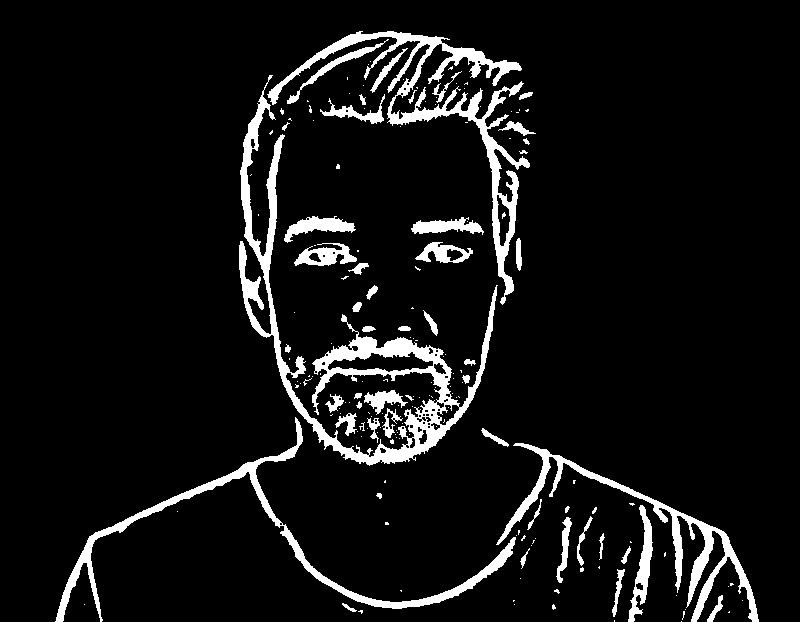
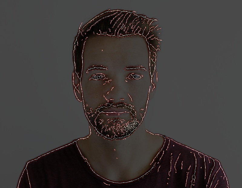
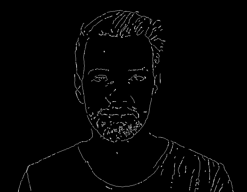
This final stage demonstrates the integrated success of the drawing pipeline.

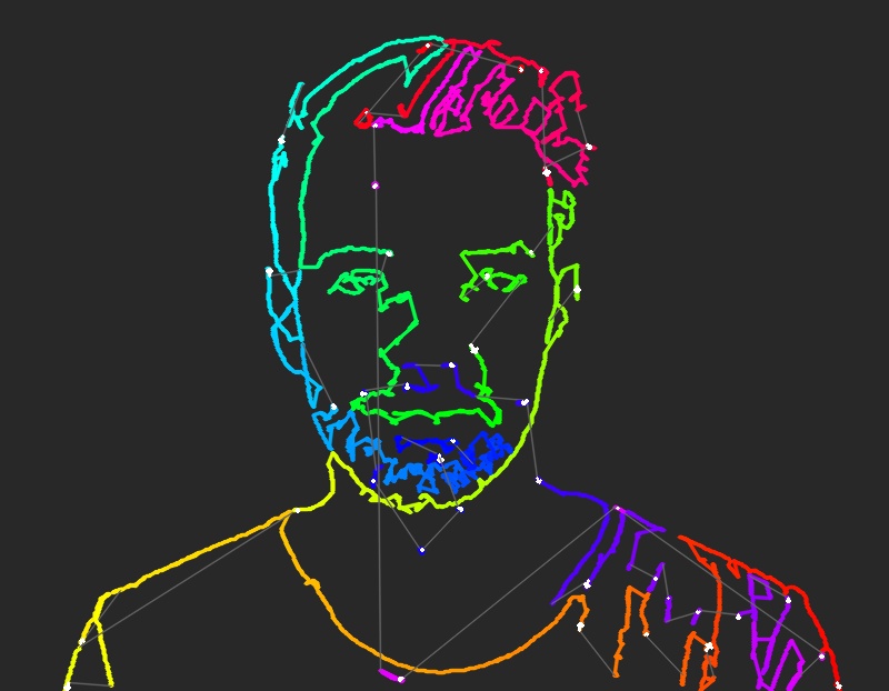
Trajectories Extracted from Contour

This is the trajectory generated from the detected contours. It represents the final path the robot will follow after completing all image processing, skeletal extraction, and adaptive smoothing stages, ensuring a kinematically feasible route for the manipulator.

Actual Robot Drawing along the Trajectory

Controlled by the QP-based IK solver and optimized Dynamixel PID gains, the robot reproduces the complex contours of the input image

---